Chapter 3: Mechanics Experiments
Conservation of Mechanical Energy
References
Crummett and Western, Physics: Models and Applications,
Sec. 8-3,4
Halliday, Resnick, and Walker, Fundamentals of Physics (5th
ed.), Chapter 8
Tipler, Physics for Scientists and Engineers (3rd ed.), Sec.
6-6,7
Introduction
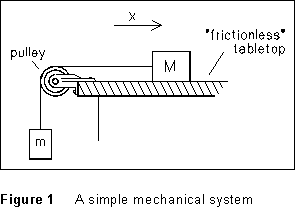 Figure 1 shows
a very simple mechanical system which we are going to examine from the
point of view of transformations and conservation of mechanical energy.
An object of mass M rests of a tabletop; it is connected by a light
string which passes over a pulley and attaches to a second mass m,
which hangs free. We will assume that friction at the contact between M
and the tabletop, and in the axle of the pulley, is so small that we can
neglect it.
Figure 1 shows
a very simple mechanical system which we are going to examine from the
point of view of transformations and conservation of mechanical energy.
An object of mass M rests of a tabletop; it is connected by a light
string which passes over a pulley and attaches to a second mass m,
which hangs free. We will assume that friction at the contact between M
and the tabletop, and in the axle of the pulley, is so small that we can
neglect it.
As mass M moves from left to right in the diagram, mass m
is rising, increasing its gravitational potential energy; and x
is increasing. M does not move vertically, so it does not come into
the potential energy calculation. Thus the potential energy of this system
is
 (1)
(1)
(U always contains an arbitrary constant.) x0
is any reference point I might choose; x = x0
is the point at which we define potential energy to be zero. If the string
connecting the mass does not stretch, the two masses are both moving at
speed v, and
 (2)
(2)
If friction in the system is negligible, the sum of potential and kinetic
energy is a constant of the motion:
 (3)
(3)
As the mass M moves from left to right, U is increasing,
so K must be decreasing, and the motion is slowing. At some
point all the system's kinetic energy has been turned into potential
energy: the system comes instantaneously to rest, then turns around and
starts transforming U back into K -- that is, it moves back
to the left with increasing speed.
On the other hand, if there is appreciable friction in the system,
it will do negative (always negative!) Work on the system, and the total
mechanical energy E will decrease monotonically as the motion goes
on. The frictional force f, if any, can be considered constant,
and
 (4)
(4)
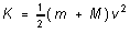
In the laboratory, you'll set up a situation closely equivalent to that
of Figure 1. An air track approximates a frictionless horizontal surface,
with a glider moving along it for mass M. Hanging mass m
is connected over to it by a thread that passes over a pulley. The goals
of the experiment are to see if Equation (3), conservation of total mechanical
energy, is borne out in this system; and to investigate the frictional
forces in the system, if frictional losses are observable.
Equipment
- Air track and gliders
- Laptop computer (yours) running kinematics software
- Various masses
- Pan balance, meter stick, etc.
Procedure
The translation of Figure 1 into the laboratory is sketched in Figure
2 above. Note: Before beginning this experiment, you should already
have completed the orientation exercise on the Sonic Ranger and the PC
which appears at the beginning of this chapter.
(1) In this laboratory you will again be recording the position
of an air-track glider using the sonic ranger. Position the sonic ranger
a little beyond the end of the air track that is nearest the wall. Put
a glider on the air track, turn on the blower (air output at position 3),
and collect data with the SR. Adjust the SR until it can reliably "see"
the glider all the way to the pulley end.) If necessary, level the track
as best you can, by adjusting the screws in the feet of the track.
(2) After the track is level, turn off the air supply. Record
the ambient temperature (there is a thermometer on the wall of the laboratory)
and calibrate the sonic ranger.
(3) You are now ready to collect data for motion of the system
of Figure 1. Attach a thread to the hanger, run the thread over the pulley
at the end of the track, and hang a small hanger on the end. Measure the
mass of your glider (leave the string attached) using the triple-beam balance;
and also measure the masses of any weights you will use for m. Record
these values in your lab notebook. Your goal is to record the motion of
the system with at least three different values of mass (m) hanging
on the end of the string. The mass values can range anywhere from 5 g to
30 g or more, depending on what masses are available.
(4) Pick one of the mass values you are going to use. Hang the
mass on the end of the string. Place the glider at the end of the track
farthest from the SR. Start the data collection and then gently
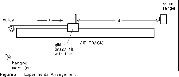
push the glider toward the SR. Check the collected data to insure that
it is clean and looks reasonable. You should see a parabolic "U"
shape, as in Figure 3.
 If you didn't catch
the returning glider, but let it bounce from the bumper, you might see
some cusps where the glider rebounds In this case, don't use data that
occurred after the glider rebounds. Oscillations occur in the pulley support
when the glider bounces; this is particularly noticeable when heavier masses
are used.
If you didn't catch
the returning glider, but let it bounce from the bumper, you might see
some cusps where the glider rebounds In this case, don't use data that
occurred after the glider rebounds. Oscillations occur in the pulley support
when the glider bounces; this is particularly noticeable when heavier masses
are used.
(5) When you have data you consider satisfactory save the selected
data to disk. Be sure to use a different name for each file you store!
Record the file name in your lab notebook, along with the mass hanging
on the end of the glider and all other pertinent information.
(6) Fit a parabola to the x vs. t data. While you are
still running the kinematics software, taking data, you can use the fitting
tools to pass a trial-and-error parabola through the data. Remember not
to look at the curve parameters until you've finished tinkering! Record
the equation of the curve.
The program will also provide you with a velocity vs. time graph.
What it does is simply (delta x)/(delta t) from the position data:
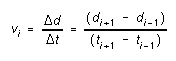 (5)
(5)
(Notice that the velocity values are internal to the software and are
not saved when you save your data to a file.) During the time interval
during which the x-t graph is parabolic, the v-t graph should
be a straight line.
(7) Repeat the acceleration measurements of (4)-(6) above for
at least two other mass values m on the end of the string.
Analysis
The goal here is to check whether the sum of potential and kinetic energies
does stay constant! Do the following for each of your data sets:
(1) Import the data set into Excel. Use Equation (5) to construct
a column of velocity data corresponding to the position data. Construct
three more columns containing the potential energy, kinetic energy, and
total energy at each time value. (In computing U, notice Figure
2: what the program records is d, the distance from the flag to
the ranger; x increases when d decreases.)
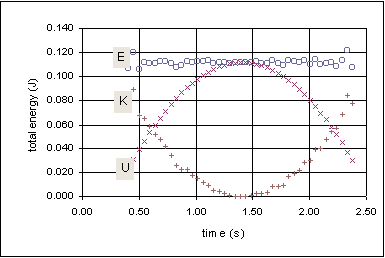 (2) Make
a graph showing the displacement of the glider vs. time; and another
graph of potential energy, kinetic energy, and the total mechanical energy
vs. time. Include these graphs for (two graphs for each of your
data sets) in your notebook at the appropriate place. (Graphs from the
data shown in Figure 3 appear at right.)
(2) Make
a graph showing the displacement of the glider vs. time; and another
graph of potential energy, kinetic energy, and the total mechanical energy
vs. time. Include these graphs for (two graphs for each of your
data sets) in your notebook at the appropriate place. (Graphs from the
data shown in Figure 3 appear at right.)
(3) Do your graphs support the idea that mechanical energy is
a constant of the motion? Comment, explain, and/or discuss.
(4) If there is a small, steady decrease in your total-energy
graph, it is probably due to frictional losses. If you observe this in
your data, try to estimate the frictional force (f) from Equation
(5). (If you do observe a measurable frictional force), does it appear
to be more or less the same in all your data sets, or does it tend to increase
with increasing m? This might tell you where (glider or pulley)
the friction is acting.
If you didn't get your track very level in Procedure (1), the vertical
motion of M might also cause a small secular change in E.
How could you discriminate between this, and a frictional force?
The Simple Pendulum
DLH/GCK 5/96 - updated 7/97